Chapter 21 – Bessel Beam Alignment of a Single Lense

Introduction: In Chapters 14 and 15 I explained how a Bessel beam is used to align optics when you have all the necessary degrees of freedom to fully align the optics in tilt, decenter and focus. Many times, you have physical constraints due to the hardware the optics are installed in, so you don’t have the ability to both tilt and decenter the optic. The question then becomes what the best is you can do, or what is the best compromise for alignment, given the constraints. This chapter explores an example of centering a single optic to understand the choices better.

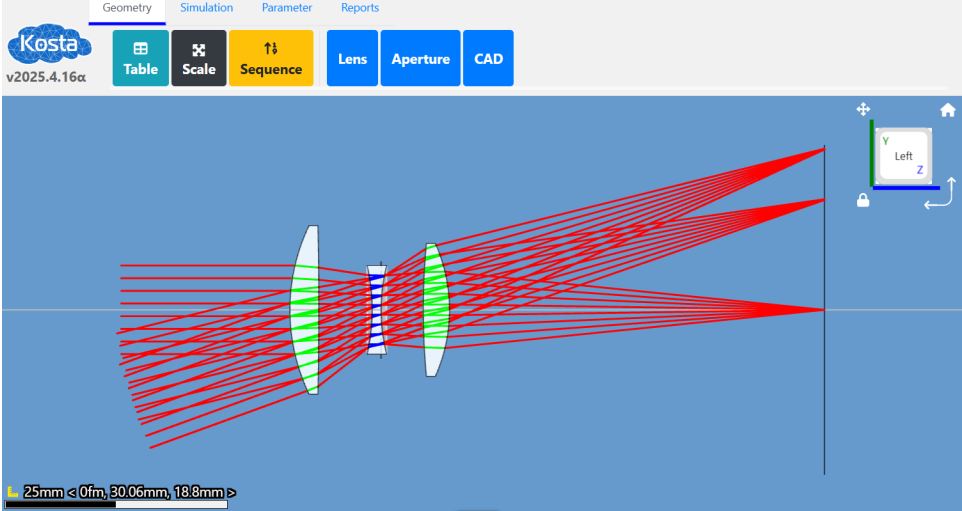
Initially I started out with a goal of trying to understand the entire assembly of the 50 mm efl Cooke triplet example in Zemax. It soon became obvious that there was a lot to learn from the centering of the very first element. The Cooke triplet example looks like Fig. 1 as shown in the KostaCloud optical design software I used.

Since the negative element is the smallest one it must be installed in the cell first. Depending on how the cell is designed, then one or the other positive elements are installed, and the cell inverted to install the remaining element. To make this a realistic example I assumed the negative element was edged to have a flat annulus on the side which would sit on the seat in the cell. Further, I assumed this flat annulus was tilted 1 milliradian (about 3 minutes of arc), a typical catalog optics tolerance for edging. It quickly turned out this little error made the resulting errors so small that it was difficult to see what was happening, so I increased the tilt to 10 mrad, about ½ a degree.

After centering the negative element, I went on to install the rear element, and it soon became obvious that to explain the whole process was going to get complex. This is why I backed off and decided to show in detail what was happening when I centered just the negative element. The other reason to keep this simple is that I want to contrast the Bessel beam method with that of using a rotary table to do the centering and this is a good example for doing that.

Centering a single optic: Fig. 2 shows just the negative element tilted 10 mrad and the optical axis as the line joining the centers of curvature of the two surfaces. Even this picture does not show all the details because the different centering conditions are so close together it is impossible to see without zooming in.

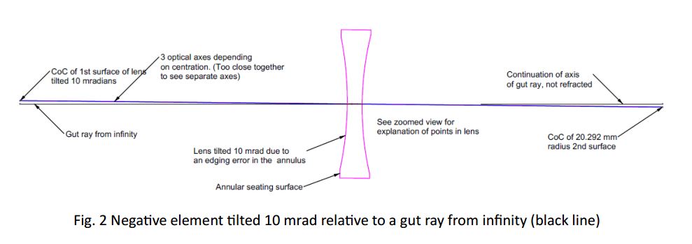
The optical axis of the tilted lens is the line joining the two centers of curvature and the axis is rotated about the 1st surface (left) of the lens. The optical axis line looks a little fuzzy because it shows the optical axis in 3 different positions depending on how we center the lens. We will discuss this below, but first I want to describe how the lens will be centered using a Bessel beam.

A Bessel beam is projected from the left in Fig. 2 along what I have called a gut ray from infinity. I am assuming a perfect cell seat that is perpendicular to the gut ray and that the lens annulus is sitting on this seat perfectly with no contamination, burrs or other disturbances to a perfect match.

I put a detector to the right of the lens to sense the Bessel beam. In my lab, I use the Point Source Microscope (PSM) as the detector, but any similar device will work. In my example I place the focus of the PSM 10, 100 and 1000 mm from the second surface of the lens, and each time center the PSM on the Bessel beam before placing the lens on the seat. When the lens is initially installed in the simulation it is perfectly centered to the gut ray but always has the 10 mrad tilt. The tilt causes the Bessel to shift and tilt as shown in Table 1.

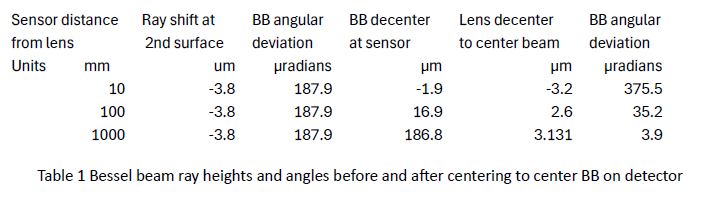
Independent of where the detector is located, Table 1 shows the ray shift and ray angle leaving the lens remains the same as for the centered but tilted lens. However, to center the Bessel beam on the detector the amount of decenter goes from -3.2 µm to 3.131 µm at 1 m. Because the distance to the detector is greater the angular deviation is less the farther the detector is from the lens. If the detector were at infinity, the amount of decenter to center the beam on the detector would 3.8 µm, the shift of the ray going through the tilted lens. This is the same beam shift, or offset, one would expect getting from a plane parallel window of the same thickness and index.

Magnified view of Bessel beam paths: Looking at just the negative element, it is easier to see where the Bessel beam crosses the reference axis for different amounts of decenter to correct for the tilt of the lens, see Fig. 3.

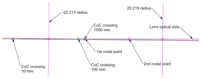
Fig. 3 Zoomed section of negative element showing nodal points and Bessel beam intersections the lens optical axis

Even with this magnified view it is difficult to see what is happening without some explanation. The two vertical arcs are the lens surfaces surrounding the optical axis. The nodal points are shown inside the lens. For the lens centered so the Bessel beam is centered on the detector at 10 mm from the lens, the Bessel beam crosses, or intersects, the lens optical axis to the left of the lens’ first surface, the blue circle. When the lens is centered to make the beam centered on the detector at 100 mm, the intersection is the green circle to the left of the 1st nodal point.

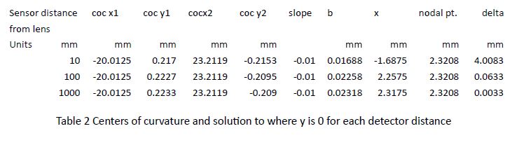
When the lens centration is such that the beam is centered on the detector at 1000 mm, the Bessel beam intersection is the red circle just 3.3 um to the left the nodal point. This means that the lens is centered to within 3.3 um x 0.01 radians = 33 nm of the optical axis when the position of the Bessel beam is centered on the detector. Even at 100 mm from the lens, the optical axis is within 0.6 um at the nodal point. To see this better refer to Table 2.

Clearly, every lens with different powers and shape factors will behave slightly differently, but the trend is obvious. The results in these two Tables are combined in Table 3.

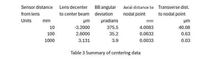
If the tilted lens is decentered to make the Bessel beam fall on the center of the detector 1000 mm away the beam exiting the lens has an angle of 3.9 µradians with respect to the optical axis and is within 33 nm of the optical axis transversely at the nodal point. For all practical purposes this is perfect alignment.

Conclusion: We have shown how to achieve perfect alignment to practical limits of precision using simple x-y motion and immediate feedback on the accuracy of alignment. The simplicity of the method opens the possibility of automating alignment. The insights gained by this example provide a direction for examining the next steps of adding the other optical elements to the lens assembly. We will look at this in the next Chapter.